We now use the assumptions stated earlier to establish the major
statistical properties of OLS estimates within the framework of the LRM.
Assumption A6 introduces a new parameter, the variance of the disturbance
terms  . This is another unknown population parameter which must
be estimated from the data. Since the prediction error
  is analogous
to the actual disturbance term
  , it might make sense to estimate
the variance of the u's with the (observable) variance of the prediction
errors.
We already know from the first normal equation
that the OLS prediction errors have a (sample) mean of 0. Their sample
variance equals therefore equals

The reason for dividing by N-2 rather than N will be made clear later.
Intuitively, the reason for dividing by N-2 is that two parameters must
be estimated to compute the error terms ( and
and  ). When
computing the sample variance of a variable, it is typical to divide by
 because one parameter (the sample mean) must be estimated to
compute the sample variance. This changes the degrees of freedom in the sums of squares
that defines
  .
.
Each of the following properties is derived in class.
- 1. Properties Requiring Assumptions
A0 through A4
- OLS estimates are unbiased
estimates of
 ,
,  , and
, and  .
.
- 2. Properties Requiring Assumptions A0-A4
and A5 and A6.
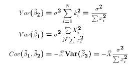
- The true Variances of the OLS estimates take the form:

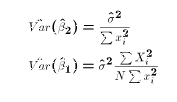
- Since the true variances include the unknown population parameter
 , it is necessary to estimate the variances by inserting
the estimate of
  :
:

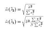
- The estimated standard errors are simply defined as the square roots
of the respective variances of the OLS estimators:

- Gauss-Markov Theorem:
- Under Assumptions A0-A6, OLS estimates are the Best (lowest variance)
Linear Unbiased Estimates of
 and
and  .
.
-
- 3. Properties Requiring Assumptions
A0 through A6 and A7
- OLS estimates are normally distributed:

-

- The OLS estimates of
 and
and  are statistically independent
of
  .
.
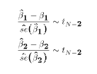
- The two ratios:

This property follows directly from the three previous properties and
the definition of the t distribution.

 and
and  ). When
computing the sample variance of a variable, it is typical to divide by
 because one parameter (the sample mean) must be estimated to
compute the sample variance. This changes the degrees of freedom in the sums of squares
that defines
  .
.
 . This is another unknown population parameter which must
be estimated from the data. Since the prediction error
  is analogous
to the actual disturbance term
  , it might make sense to estimate
the variance of the u's with the (observable) variance of the prediction
errors.