 and
and  from the sample
information. There are many ways to approach the problem of estimation in
the context of the LRM. But under our assumptions, they usually end up
pointing toward very similar solutions. Under different assumptions,
however, various approaches to estimating the PRE can give very different
results.
 and
and  of
of  and
and  , define the following terms
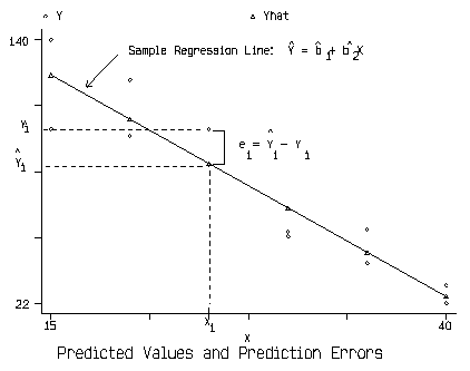
- Predicted value of $Y_i$:

- Prediction error:

- Sum of Squared Errors(SSE, also called RSS)

- The Ordinary Least Squares estimates of
 and
and  are
defined as
- the particular values
 and
and  of
of  and
and  that minimize SS for the sample data.
Graphical Representation of OLS Terminology

The Week 3 tutorial gives you a chance to experiment with fitting a linear line to a sample.

Note Because we won't be considering other estimators
for several weeks, the superscript OLS will be dropped. Unless noted
otherwise  refers to the OLS estimate of
  . Likewise
for
  .
.
The solutions come from solving the two normal equations

which in turn are simply the first order conditions for minimizing SSE.
Stata also reports the SSE in the output table, although it calls the SSE
the Residual Sum of Squares or (RSS). The interpretation of all values in
the table will become apparent as we go along.
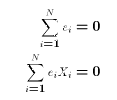
Each of these properties spring directly or indirectly from the normal
equations.


 , and
, and  . These two properties of the OLS weights
  will prove useful
in proving the Gauss-Markov Theorem later on.
The top part of this example shows you how you could use Stata as a
calculator to compute OLS estimates from data. Each "generate" statement
is a step towards the formulas for the OLS estimates. However, once
you understood what the formulas mean there is no need to compute OLS
estimates in this way. Stata does it automatically with its "regress"
command. If you look at the "Coef." column you see the match up
to the b1hat and b2hat values. The estimated coefficient on X is
*
*  Calculating OLS estimates of regression coefficients
*
. input X Y
      X    Y
  1.  1   .75
  2.  2   2.25
  3.  3   4
  4.  4   2.5
  5.  5   5.5
  6. end

. egen xbar = mean(X)                   Computes mean of X, puts in xbar
. egen ybar = mean(Y)
. gen x = X-xbar                        Generates deviation from mean
. gen y = Y-ybar
. gen xsq = x*x                         Generates deviation squared
. egen sxsq = sum(xsq)                  Generates sum of squared deviations
. gen k = x/sxsq                        Generates weight on Y
. gen kY = k*Y
. egen b2hat = sum(kY)                  Generates b2hat (OLS estimate)
. gen b1hat = ybar - b2hat*xbar         Generates b1hat (OLS estimate)
. gen Yhat = b1 + b2hat*X               Generates Predicted Y (on OLS line)
. gen e = Y - Yhat                      Generates prediction error or residual
. gen esq = e*e                         Generates OLS error square

. list, nodisplay noobs

 X   Y   xbarybar  x    y   xsq sxsq   k      kY  b2hat b1hat Yhat    e    esq
--- ---- -------- ---  ---- --- ----  ----  ----- ----- ----- -----  ----- ----
1.0 0.75 3.0 3.0 -2.0 -2.25 4.0 10.0 -0.20 -0.150 0.975 0.075 1.050 -0.300 0.09
2.0 2.25 3.0 3.0 -1.0 -0.75 1.0 10.0 -0.10 -0.225 0.975 0.075 2.025  0.225 0.05
3.0 4.00 3.0 3.0  0.0  1.00 0.0 10.0  0.00  0.000 0.975 0.075 3.000  1.000 1.00
4.0 2.50 3.0 3.0  1.0 -0.50 1.0 10.0  0.10  0.250 0.975 0.075 3.975 -1.475 2.17
5.0 5.50 3.0 3.0  2.0  2.50 4.0 10.0  0.20  1.100 0.975 0.075 4.950  0.550 0.30

. regress Y X

  Source |       SS       df       MS                  Number of obs =       5
---------+------------------------------               F(  1,     3) =    7.88
   Model |     9.50625     1     9.50625               Prob > F      =  0.0674
Residual |     3.61875     3     1.20625               R-square      =  0.7243
---------+------------------------------               Adj R-square  =  0.6324
   Total |      13.125     4     3.28125               Root MSE      =  1.0983

------------------------------------------------------------------------------
       Y |      Coef.   Std. Err.       t     P>|t|       [95 Conf. Interval]
---------+--------------------------------------------------------------------
       X |       .975   .3473111      2.807   0.067      -.1302989    2.080299
   _cons |       .075   1.151901      0.065   0.952      -3.590862    3.740862
------------------------------------------------------------------------------
 and the coefficient on the constant (=1) is
  . Notice that
when computing OLS estimates Stata never knows the true
population parameters. So "Coef." is short for "OLS Coefficient Estimates".
Compare the estimated coefficients from the regression
above to the earlier analysis
of the conditional expectation
of cigarettes. Can you use equation E7 to explain the
connection?
. gen female = dvsex - 1           * dvsex was coded 1,2 not 0,1
. regress cigs female

  Source |       SS       df       MS                  Number of obs =     600
---------+------------------------------               F(  1,   598) =    4.33
   Model |      403.44     1      403.44               Prob > F      =  0.0378
Residual |  55669.2533   598  93.0923969               R-squared     =  0.0072
---------+------------------------------               Adj R-squared =  0.0055
   Total |  56072.6933   599  93.6105064               Root MSE      =  9.6484

------------------------------------------------------------------------------
    cigs |      Coef.   Std. Err.       t     P>|t|       [95 Conf. Interval]
---------+--------------------------------------------------------------------
  female |      -1.64   .7877918     -2.082   0.038      -3.187175    -.092825
   _cons |   6.533333    .557053     11.728   0.000       5.439315    7.627351
------------------------------------------------------------------------------
This document was created using HTX, a (HTML/TeX) interlacing program written by Chris Ferrall.
Document Last revised: 1997/1/5
