
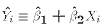
For a sample observation we have already defined the predicted value:
 . Often we may use the OLS
estimates to predict the value of Y for a a value of X that is not in the
sample. Furthermore, we will want to know how precise our prediction for
the value of Y is, whether in sample or out of sample.
. Often we may use the OLS
estimates to predict the value of Y for a a value of X that is not in the
sample. Furthermore, we will want to know how precise our prediction for
the value of Y is, whether in sample or out of sample.
Let us then consider the problem of predicting the value of Y for an
arbitrary value of X denoted  . This value of X may or may not be in
the sample used to estimate the regression equation. We can actually
think of two numbers we would want to predict for
:
. This value of X may or may not be in
the sample used to estimate the regression equation. We can actually
think of two numbers we would want to predict for
:
Individual Value: 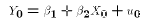
and
Mean Value![$E[Y_0 | X_0] = \beta_1 + \beta_2 X_0$](../images/reg177.gif)
Notice the difference between the two. One is the actual value of Y for
a particular observation, including that observations error term  .
The second object is the expected value of Y conditional on knowing the
value of
. For example, suppose you are a criminologist who has
estimated the following regression:
.
The second object is the expected value of Y conditional on knowing the
value of
. For example, suppose you are a criminologist who has
estimated the following regression:
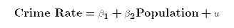
using data on city sizes and crime rates. You obtain estimates
 and
and  and then wish to make predictions about
crime rates for cities that you do not know the crime rate for. You
might want to predict the crime rate for a particular city, say Toronto,
whose population would give it a value
and then wish to make predictions about
crime rates for cities that you do not know the crime rate for. You
might want to predict the crime rate for a particular city, say Toronto,
whose population would give it a value 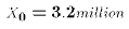 . That would
be a an individual prediction. On the other hand, you may want to know
what your model predicts is the crime on average in cities of
size 3.2 million. That would be a mean prediction. In effect, you want
to average out the effect of the disturbance terms
. That would
be a an individual prediction. On the other hand, you may want to know
what your model predicts is the crime on average in cities of
size 3.2 million. That would be a mean prediction. In effect, you want
to average out the effect of the disturbance terms  .
.
The OLS prediction is the same for both mean and
individual predictions:
![$$\eqalign{\hat Y_0 | X_0 \equiv \hat\beta_1 + \hat\beta_2 X_0\cr \hat{E}[ Y_0 | X_0] \equiv \hat\beta_1 + \hat\beta_2 X_0\cr }$$](../images/reg310.gif)
The predictions are the same because the expected value of
(that
is, the disturbance term for a particular observation such as Toronto) is
0. So one would use the OLS regression line to predict out of sample as
well as in sample. We can think of the difference the following way:
![$$\hat Y_0 | X_0 = \hat{E}[Y_0 | X_0] + E[u_0 | X_0] = \hat{E}[Y_0 | X_0]$$](../images/reg183.gif)
This equation suggests that the difference between the predictions lies in
their variance. The precision of an individual prediction is lower
because the variance of the disturbance must be taken into account.
![$$\eqalign{Var(\hat{E}[Y_0 | X_0] &= Var(\hat\beta_1 + \hat\beta_2 X_0) \cr &= Var(\bar Y) + (X_0-\bar X)^2Var(\hat\beta_2)\cr &= \sigma^2\biggl( {1\over N} + {(X_0-\bar X)^2 \over \sum x_i^2} \biggr)\cr} $$](../images/reg311.gif)
Notice that variance increases the farther the value of
is from the
sample mean of X. It is at the sample mean of X that we have the most
information about the relationship between X and Y. As we move away from
that point, the less information we have and the more unsure we are of
the location of the population regression line.
Since we assume that the disturbance term is unrelated to the value of
 , we can see that
![$$Var(\hat Y | X_0 ) = \sigma^2 + Var(\hat E[Y_O | X_O]) = \sigma^2\biggl( 1 + {1\over N} + {(X_0-\bar X)^2 \over \sum x_i^2} \biggr)$$](../images/reg312.gif)
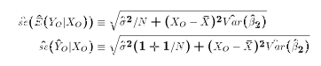
Of course we can't directly compute the variance in our predictions,
because they depend upon the value of  . As usual, we can only
compute the estimated variance and standard deviation of the
prediction.
. As usual, we can only
compute the estimated variance and standard deviation of the
prediction.
Note that under A7 both predictions are normally distributed, so that we can compute confidence intervals and perform hypotheses tests on actual values of Y and E[Y].
Once we know the formula for the variance of the prediction we are
making, the formula a confidence interval for the prediction is the same
as usual:
![$$\eqalign{\hat{Y}_O | X_O &\pm \hat{se}(\hat Y_O) t_{N-2,1-\alpha}\cr \hat{E}[Y_O|X_O] &\pm \hat{se}(\hat E) t_{N-2,1-\alpha}\cr} $$](../images/reg313.gif)
where
To compute the confidence interval by hand using only the regression
output requires five numbers:
5 Pieces of Information to Compute Confidence Intervals for Predictions
All but  (the value to predict for, chose by you)
(reported as Mean Squared Error in the table)
(the value to predict for, chose by you)
(reported as Mean Squared Error in the table)

 (sample mean of X, which requires use of the
summarize command)
(sample mean of X, which requires use of the
summarize command)
 (square of estimated standard error)
can taken directly off the Stata regression output.
Stata also has a built in predict command that computes
predictions and standard errors of predictions. Learn more about them in
the Week 4 tutorial.
(square of estimated standard error)
can taken directly off the Stata regression output.
Stata also has a built in predict command that computes
predictions and standard errors of predictions. Learn more about them in
the Week 4 tutorial.
This document was created using HTX, a (HTML/TeX) interlacing program written by Chris Ferrall.
Document Last revised: 1997/1/5