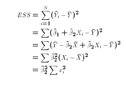
In other words, ESS depends only the values of X and
 .
.
 . This is the total variation in the OLS
prediction errors in the sample. (Since we know the mean error
is 0, then RSS is the sum of squared deviations from the mean.
There are two other variations that are useful to define in the
LRM:

 . Therefore,
ESS is also a "sum of squared deviations from mean" as is TSS and RSS.
In other words, ESS is how much the predicted values in the sample vary,
while TSS is how much the actual values vary. Note:
The Stata output table for a regression
refers to "ESS" as "Model Sum of Squares"
Let us derive a formula for ESS:

In other words, ESS depends only the values of X and  .
.
With a little bit of algebra we can go on to show
TSS = ESS + RSSThat is, the OLS estimates of the LRM decompose the total variation in Y into an explained component (explained by X) and an unexplained or residual component. The Stata regression output table shows this analysis of variance by reporting TSS, ESS, and RSS.
Notice that under A7, each Y observation as well as the sample mean of Y
are normally distributed. Therefore  is normally
distributed. TSS is therefore a sum-of-squared normal variables with mean
0. To calculate TSS, one needs to have calculated
  , which imposes
one linear restriction on the deviations. The degrees of freedom
associated with TSS are therefore N-1. We have already
argue that to calculate RSS requires two restrictions embodied in the two
OLS normal equations. The degrees of freedom associated with RSS is
N-2. What about ESS? Under assumptions A0-A7
 is normally distributed, and ESS depends only on its value.
Even though ESS is defined as the sum of N normal variables, there are N-1
dependencies among them. ESS is therefore associated with a chi-squared
random variable with 1 degree of freedom.
This leads us to the conclusion that OLS not only decomposes the
variance in the Y observations, it only decomposes the
degrees of freedom in the variation:
   N-1          =       1          +       N-2
D.of F. for TSS = D. of F. for ESS + D. of F. for RSS
The preceding discussion of the analysis of variances leads quite easily
into a measure of how well the OLS estimates fit the sample data. First,
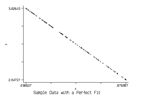
imagine a data set in which all the values of X and Y line up on a line:

In this case, OLS will minimize the squared errors and will recover the
line. The predicted values for each observation will be identical to
the actual values:  for all i. The OLS estimates would
perfectly fit the data. Or, in other words, RSS = 0. But then
this must mean that TSS = ESS: all the variation in Y is explained by
the linear regression model.
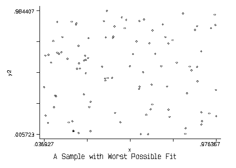
Now take the other extreme in which there is no correlation between X and Y in the sample. The sample is simply a flat cloud of points:

In this case, the OLS estimate would lead to:  , and
, and
 for all i. Notice that if
  , then
ESS = 0. That is, none of the variation in Y is explained by variation
in X. Therefore TSS = RSS, all the variation is left unaccounted for by
the model. This would be the worst fit of the data.
If we assign a "1" to a perfect fit and a "0" to the worst fit, then all other cases should lie somewhere in between. X should explain some of the variation in Y, but generally not all of it. A logical measure of fit would therefore be:
R² = Measure of fit = ESS /TSS
This ratio is usually referred to as R² or "R-squared". The
interpretation is simple:
R² is the proportion of total variation in Y in the sample explained by the OLS regression line. It is a rough measure of how close the sample data lie to the estimated regression line.R² in and of itself does not tell us anything about whether the LRM is correct. A poor measure of fit does not imply a poor model. It could be that the fit is poor (low value of R²) simply because many other factors help determine Y (high value of
 ). Conversely, a good
measure of fit does not imply a good model. One can have a good fit (high
R²) and have a very dumb and misleading model. For example
regressing a person's weight in kilograms on a person's weight in pounds
will lead to a perfect fit. But the result doesn't tell us anything about
weight. It only tells us that we properly converted from kilograms to
pounds (or vice versa). Believe it or not, it is not uncommon for people
to report results almost as silly as this.