
Would an increase in the minimum wage increase unemployment among low-wage workers?
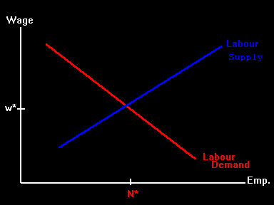
The competitive equilibrium looks like the following:
 acts as a price floor within this simple model.
If the minimum wage is not binding
acts as a price floor within this simple model.
If the minimum wage is not binding  , then it should have no effect
on employment or unemployment. A binding minimum wage has the following
effect:
, then it should have no effect
on employment or unemployment. A binding minimum wage has the following
effect: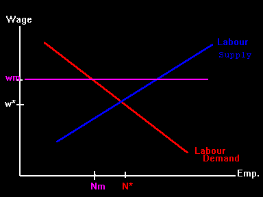
(Note: the upward sloping line should be labeled Labour Supply.) The result is a lower level of employment (Nm), or higher rate of unemployment. Of course, not everyone works at a minimum wage. We need to interpret this as the market for low-skill (low-wage) workers, such as teenagers who have dropped out of high school.
where u captures
determinants of labour demand: technology, output prices,
prices of other factors of production, etc.
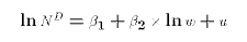
 is the quantity demanded written
as a function of the market wage w. (You should refer to your intermediate
microeconomics textbook or notes to remind yourself that a Cobb-Douglas
production function generates a demand function of the form (D1).)
is the quantity demanded written
as a function of the market wage w. (You should refer to your intermediate
microeconomics textbook or notes to remind yourself that a Cobb-Douglas
production function generates a demand function of the form (D1).)
. If
the price floor is not binding, then N is found at the intersection of
labour demand and labour supply. Even if they are both simple
log-linear curves, the market outcome N would demand upon four parameters.
With a price floor, we can focus attention upon one equation and
two unknown parameters.
 . Since the values of
 and
and  depend upon unobservable things such as production
functions, these values are unknown constants or
perhaps population parameters.
(Even if we assume that we know the form of the demand curve we
aren't so bold as to assume the slope and intercept.)
(and through it unemployment)
responds to the minimum wage depends upon the slope of the demand curve:
depend upon unobservable things such as production
functions, these values are unknown constants or
perhaps population parameters.
(Even if we assume that we know the form of the demand curve we
aren't so bold as to assume the slope and intercept.)
(and through it unemployment)
responds to the minimum wage depends upon the slope of the demand curve:
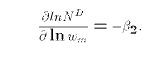
Recalling the definition of supply elastiticity, we see that
is
the elasticity of the demand curve. Economic theory predicts that
 (downward sloping demand curve). So since
our initial question concerns a change in the
mininum wage we can focus on not two unknown parameters but only
one unknonwn parameter. We therefore can re-form our
initial question into a much easier question:
(downward sloping demand curve). So since
our initial question concerns a change in the
mininum wage we can focus on not two unknown parameters but only
one unknonwn parameter. We therefore can re-form our
initial question into a much easier question:
How big is
 and employment rates
  ,
where
,
where  is an index the different labor market.
According the demand-curve model, the relationship between the two
values depends upon the other factors operating in the market,
which we might call
is an index the different labor market.
According the demand-curve model, the relationship between the two
values depends upon the other factors operating in the market,
which we might call  .
.
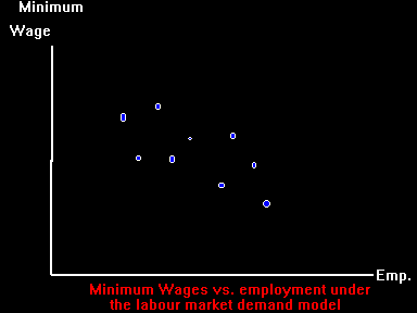
In other words, the slope of the supply curve causes the cloud of
observations to be downward sloping as long as the influence of other factors
is small relative to the slope. But if the variation
in
is relatively large (or the variation in mininum wages
is relatively small) the cloud of points might appear flat even though
is less than zero.
Using sample information, can we isolate the slope
and
from data. Instead,
we must estimate the
unknown population paramter
from data on a
sample of employment rates and minimum wages.
be called  .
Based on
, it is simple to form the prediction:
.
Based on
, it is simple to form the prediction:
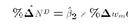
If a politician told you how much the mininum wage was going to change, you could could plug into this formula and predict for him/her the percentage change in
. So the easy part of the job is
carrying out the prediction. The hard part is coming up
with an estimate of
in the first place.
is a
random variable
(it depends on sample information which includes the effect of the
disturbance factor u), your prediction  is
also a random variable.
Your prediction about the effect of
changing the mininum wage is itself an estimate. You, and
most definitely your client or audience, will ask the further question:
is
also a random variable.
Your prediction about the effect of
changing the mininum wage is itself an estimate. You, and
most definitely your client or audience, will ask the further question:
How precise is a prediction based on the estimateWanting to know how precise your estimate is trying to infer something about the actual change based on your prediction. You might be asked to form a confidence interval for the actual employment response. Or, you might be asked to test the hypothesis that there is no employment response, which is the same as testing the hypothesis that
is zero.
- We begin by asking a specific policy question about the effect of raising the mininum wage.
- Using basic economic theory and some simplifying assumptions (like log-linear demand), we reduced the question to asking a specific numerical question about one theoretical construct, the slope of the demand curve for low wage workers.
- We then realized that finding this value requires us to ask a specific statistical question about estimating a slope from a cloud of points.
- If we are successful in carrying out this step, then we are lead to ask a specific inferential question about how precise our estimate is.
- The goal of econometrics
To use statistical techniques to estimate and test economic models using economic data.