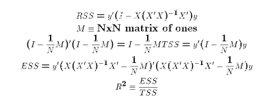
if the data do not contain all the data then one cannot compute all of the OLS estimates, so violation of this assumption is fatal to estimating the full model.
there are many reasons to think about how the form of the Population Regression Equation may be wrong. Perhaps one is not sure that the PRE should be linear, log-linear, or some other transformation of the original data. Even worse, perhaps the relation between Y and X can't be linearized at all. That is one way to think about the logit and probit models - as extensions of the OLS model in which the relationship between Y and X is a specific one that cannot fit into the LRM framework.
If the PRE did not generate the sample information then some other process did. So violation of these assumptions is in many respects equivalent to the violation of A1.
As mentioned in the original discussion of the assumptions,
A3 is really a technical assumption. If E[u] is not zero then one can
re-define
Recall that under A0-A4 OLS estimates are unbiased estimates of the
LRM parameters. Violating Assumptions A0-A3 leads to either trivial
changes (in the case of A0 and A3) or fairly esoteric statistical
issues of what model seems to be generating the data. I call this
esoteric because it tends to lead one away from the economic
content of the LRM, unless one looks for other specifications
that come from economic theory. However, most analysis of violations
of A1 and A2 are not based on economic theory.
Violation of A4/A4* is another matter altogether. If cov(u,X) is not
0 (the A4* way of seeing it), or if one cannot think of X as "exogenous" to
Y (the A4 way), then one is in trouble. And this trouble has a lot
to do with economic theory. A whole chapter on IQ scores
is devoted to explaining why A4 is a critical assumption.
Traditionally one would go from this point to study ways to "fix" OLS
estimates when A5 and A6 do not hold. But it is important that
these assumptions only enter at the point of deriving
Since OLS estimates are linear in the Y's, violation of
the normality assumption is really only a problem in small samples.
That's because for values of N larger than 30 the Central
Limit Theorem begins to kick in. That is  to include the mean of u.
 .
This means estimated standard errors and confidence intervals won't
be good if A5 and/or A6 is not true. However, this is in many ways
a much smaller problem than having either a non-linear model or
not even having unbiased estimates. Therefore, our discussion of
these assumptions is brief.
 will be
asymptotically normally distributed even if u is not normally
distributed.

 be the vector you want to
predict for. Then following the earlier discussion the mean and
individual predictions are the same,
![$$\eqalign{\hat E[ Y_0 | X_0] &= X_0\hat\beta\cr \hat Y_0|X_0 &= X_0\hat\beta\cr}$$](../images/mul275.gif)
![$$\eqalign{ Var(\hat E[Y_0]) &= {X_0}' Var(\hat\beta) X_0 = \sigma^2 {X_O}'(X'X)^{-1}X_O\cr Var(\hat Y_0) &= {X_0}' Var(\hat\beta) X_0 + \sigma^2\cr }$$](../images/mul276.gif)
![$$\eqalign{ \hat{Var} (\hat E[Y_0]) &= \hat\sigma^2 {X_0}' (X'X)^{-1} X_0\cr \hat{Var} (\hat Y_0) &= \hat\sigma^2\bigl( {X_0}' (X'X)^{-1} X_0X_0+1\bigr) \cr }$$](../images/mul277.gif)
