
A random matrix is a matrix of random variables. For example the vector of disturbance terms is a random vector since each element of the vector is a random variable. A constant matrix is, of course, a special type of random matrix in the same sense that a constant is a special case of a random variable that does not vary across points in the sample space.
The expectation of a random matrix is the matrix of expectations of each random
variable in the random vector. That is, let V be a m x r random matrix, and let
Notice that m does not have to equal r. That is, the transformation matrix A may
change the dimensions of the random matrix. AV is a n x r random matrix, not a m x
r. The proof of this result requires you to write out what an element of the matrix
AV+C looks like, apply the expectation operator to it, and then see that the result
is exactly the same as if you had written out AE[V] + C.
 denote the random variable in the ith row and jth column of V. Then
![$$E[V] \equiv \left|\matrix{ E[v_{11}]&E[v_{12}&\dots&E[v_{1r}]\cr E[v_{21}]&E[v_{22}]&\dots&E[v_{2r}]\cr \vdots&\vdots&\vdots&vdots\cr E[v_{m1}]&E[v_{m2}]&\dots&E[v_{mr}] }\right|$$](../images/mul239.gif)
Note that expectation is still a linear operator when defined this way.
That is, if A is a n x m matrix of constants and C is a n x r vector of
constants, then
E[AV + C] = AE[V] + C E[ (v-E[v])(v-E[v])' ]
This generalizes the notion of covariance, which itself generalized the notion of
variance. Notice that (v-E[v])(v-E[v])' is a m x m matrix (when v is m x 1). So
Var(v) is always a square matrix. If we multiply (v-E[v])(v-E[v])' out, we can see
that the ith row, jth column of it contains
E[ (v-E[v])(v-E[v])' ]
This generalizes the notion of covariance, which itself generalized the notion of
variance. Notice that (v-E[v])(v-E[v])' is a m x m matrix (when v is m x 1). So
Var(v) is always a square matrix. If we multiply (v-E[v])(v-E[v])' out, we can see
that the ith row, jth column of it contains ![$(v_i-E[v_i])(v_j-E[v_j])$](../images/mul240.gif) . The
expectation of this scalar random variable is by definition:
. The
expectation of this scalar random variable is by definition:
![$$E[ (v_i-E[v_i])(v_j-E[v_j]) ] = Cov(v_i,v_j)$$](../images/mul241.gif)
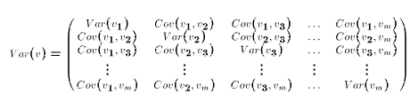
So each element of Var(v) is a covariance. The diagonal elements of Var(v) are
simply the variances of the corresponding elements of the v vector. Since Cov(r,s) =
Cov(s,r), the matrix Var(v) is symmetric. Summing this up,
 with
with
![$$Var[v] = \pmatrix{\sigma^2_1&0\cr 0 &\sigma^2_2}$$](../images/mul244.gif)
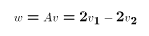
![$$\eqalign{Var[Av] = &AVar[v]A'\cr = &\pmatrix{2 & -2}\pmatrix{\sigma^2_1&0\cr 0 &\sigma^2_2}\pmatrix{2\cr -2}\cr = &\pmatrix{2\sigma^2_1 -2\sigma^2_2}\pmatrix{2\cr -2}\cr = 4\sigma^2_1 + 4\sigma^2_2\cr}$$](../images/mul246.gif)
 I
I
 and
and  .
.