
- We will define confidence intervals for a
population parameter
 in the following situation:
- We have a sample of size N
- We already have an estimator
 that we know is unbiased
- We also know from some other results that
The value of k is going to depend on the situation in which we are estimating
.
- A confidence interval for a parameter
, given
and estimator
is a range
![$R= [\hat{a}-\hat{b},\hat{a}+\hat{a}]$](../images/glo058.gif) computed
from the sample data so that the true value
lies in
computed
from the sample data so that the true value
lies in
 in a pre-determined (before sampling) percentage of
all possible samples from the population.
in a pre-determined (before sampling) percentage of
all possible samples from the population.
- The pre-determined percentage is called the confidence level. It is usually denoted by "1-
 ." where
is the significance level.
." where
is the significance level.
- Note that the range is defined by a pair of numbers
and  which by defintion are functions of a
sample, so they are random variables.
which by defintion are functions of a
sample, so they are random variables.
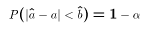
- The definition now says that
must be chosen so that
the true value
must lie in the range in 1-
of the
samples. In other words:
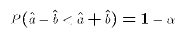
or
- The only random (sample-dependent) values in (*) are
and
. This explains why we need to know the sampling
distribution of
, otherwise we could not determine
a value of
that makes (*) true.
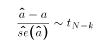
- We started with the presumption that left hand side of the inequality in (*) equals the absolute value of the numerator of a
 distribution.
Dividing both sides of the inequality by the denominator
allows us to write (*) as
distribution.
Dividing both sides of the inequality by the denominator
allows us to write (*) as
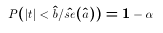
- Using tables of the t-distribution, we find the critical value
 that makes this inequality true. In
other words, set:
that makes this inequality true. In
other words, set:
where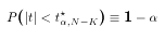
- This leads to the much more familiar expression for a confidence interval for
:
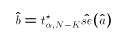
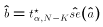
![$$R \equiv [ \hat{a}-t^\star_{\alpha,N-K}\hat{se}(\hat{a}) , \hat{a}+t^\star_{\alpha,N-k}\hat{se}(\hat{a})]$$](../images/glo295.gif)
3 Steps to construct a Confidence Interval
- Choose your confidence level 1-
,
determine the value of k for your situation (discussed later),
and look up the value of
 .
.
- Compute the estimate
and its estimated standard error
![$\hat{se}[\hat{a}]$](../images/glo071.gif) .
.
- Compute
 and finally
  .
.
Make a decision to either REJECT or FAIL-TO-REJECT a hypothesis that a population parameter equals a particular value. Do this while setting the proportion of samples in which rejection occurs when the hypothesis is true to a pre-determined value.The proportion of samples in which FALSE rejection occurs is called the level of significance of the test, usually denoted
. We also call
this the
probability of a Type I error. A Type II error is failing to reject the
hypothesis when it is actually false.When constructing a confidence interval, the interval depends on the sample and so it is random. When conducting a hypothesis test, the decision (reject or fail-to-reject) depends on the sample and so the decision made is random before the sample is drawn.
Notice that .465 is
greater than alpha = .1, which is the area
corresponding to P(|Z|>1.645).
Suppose Stata tells you the p-value of a calculate test
statistic. Looking at the figure above you should be
able to see that you can make the decision about the
hypothesis test without checking whether the calculated
value lands in the critical region or not. If the
p-value is greater than
5 Required Elements of a Hypothesis Test
Each of these required elements can be determined before
anything is done with the sample information. Once each of
these elements is specified correctly, carrying out a hypothesis
test is simple.
 , which states the value to test.
 , which are the values to test against
),
also known as the test's level of significance.
The value of
is chosen by the researcher!
, which are the values to test against
),
also known as the test's level of significance.
The value of
is chosen by the researcher!
Two Ways to do a Hypothesis Test: Use Critical Region or p-value
Why use the p-value method rather than the critical region
method? As long as the statistical package makes it easy
to get the p-value then you don't have to look up the
critical value of the test statistic as well, which saves
you time. Why doesn't a statistical package like Stata
provide critical values as well as p-values? Because
critical values depend upon your own personal choice of
To illustrate the two ways to actually make the decision
to reject or fail to reject H0, we'll take the common
example of a two-sided Z test. That is,
part 4 of the 5 required elements in this case
is a test statistic that follows the standard normal
distribution when the null hypothesis is in fact true.
Let's say you are
willing to take a one-in-ten chance that you reject
H0 when in fact it is true. That is,
= .10.
If you look up values of the z distribution you will
find that z*(.10)=1.645 in this case. (You can also
have Stata calculate this for you by typing di invnorm(.95) (yes,
.95 not .90 because this example is a two-sided test).
So part five of the five required elements would be:
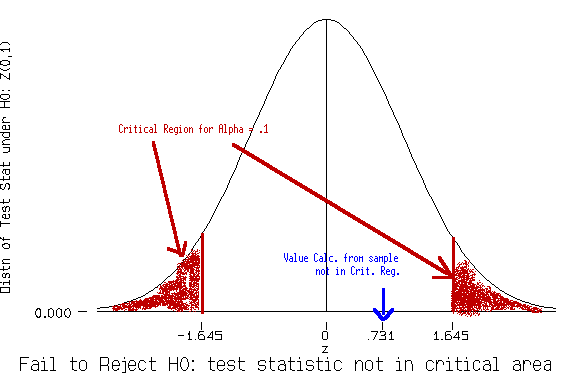
Example Crticical Region: Reject H0 if |zcalc| > 1.645.
Given your data, you calculate the test statistic and
find it equals 0.731. Therefore, you could complete this
test in the following way:
The value of the test statistic in the sample is .731.
Since |.731| is < 1.645, I fail to reject the null hypothesis.
.
Here is a picture that goes along with this decision.
 ).
).
What is a p-value? The p-value of a calculated
test statistic is the probability under H0 that the
test statistic takes on a value greater in
absolute value
than the calculated value. (For one-sided test
the appropriate p-value would
be the probability that
the test statistic takes on a value either greater
or less than the
calculated test statistic but not both. Stata usually
reports p-values associated with two-sided tests when
they are possible.)
Why is the p-value useful? Let's return to the example to see
why. With zcalc=.731 and alpha=.1 we fail to reject the
two-sided hypothesis because .731 is not in the critical
region z > |1.645|. Suppose we knew
Prob(|Z|>.731). That is, suppose we knew the area
shaded blue in the figure below:
 In fact, one can look up the area of the shaded region
using Z tables, or you can let Stata do the work by
typing
In fact, one can look up the area of the shaded region
using Z tables, or you can let Stata do the work by
typing di 2*normprob(-.731).
Either way, you find that the area of the region
equals .465. That is, there is a .465 chance that a
Z random variable will take on a value greater in
absolute value than .731.
This would be the p-value
of the calculated test statistic.
, then we know that
we should fail to reject H0. On the other
hand, if the p-value is less than
then
this means the calculated test statistic does lie in
the critical region and we should reject H0.
which the program doesn't know ahead of time. The
p-value depends only upon H0, the calculated value of the
test statistic (which comes from the sample), and whether
the test is one-sided or two-sided.
Can using p-values be confusing? Yes!. Notice
that the inequality switches when using the p-value
approach than when using the critical region approach.
That is, the decision rule Reject H0 if calculated
test statistic is greater in absolute value than the critical
value becomes Reject H0 if p-value is
less than
.
If you mix this up you will come to exactly the wrong
conclusion! Also, you must avoid comparing apples
and oranges. Whichever decision rule you choose to
apply, always compare test statistics
to critical values and p-values to significance
levels.